A Brief Review of Reinforcement Learning

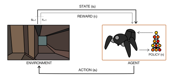
Reinforcement Learning is a mathematical framework for experience-driven autonomous learning. An RL agent interacts with its environment and, upon observing the consequences of its actions, can learn to alter its own behaviour in response to the rewards received. The goal of the agent is to learn a policy \(\pi\) that maximizes the expected return (cumulative, discounted reward).

• Background
• Value Function Algorithms
  • TD Learning
  • SARSA
  • Q-Learning
• Policy Gradient Algorithms
  • REINFORCE

Background

At each time step \(t\), the agent receives a state \(s_t\) from the state space \(S\) and selects an action \(a_t\) from the action space \(A\), following a policy \(\pi(a_t \vert s_t)\). Policy \(\pi(a_t \vert s_t)\) is the agent’s behavior. It is a mapping from a state \(s_t\) to an action \(a_t\). Upon taking the action \(a_t\), the agent receives a scalar reward \(r_t\), and transitions to the next state \(s_{t+1}\).

Transition to the next state \(s_{t+1}\) as well as the reward \(r_t\) are governed by the environment dynamics (or a model). State transition probability \(P(s_{t+1} \vert s_t,a_t)\) is used to describe the environment dynamics.

The return \(R_t = \sum_{k=0}^{\infty}\gamma^kr_{t+k}\) is the discounted, accumulated reward with the discount factor \(\gamma \in (0, 1]\). The agent aims to maximize the expectation of such long term return from each state.

A value function is a prediction of the expected, accumulative, discounted, future reward. In other words, a value function is the expected return. A value function measures how good each state, or state-action pair, is. The state value \(v_{\pi}(s)\) is the expected return for following policy \(\pi\) from state \(s\).

\(v_{\pi}(s)\) decomposes into the Bellman equation:

We are assuming a stochastic policy \(\pi(a \vert s)\) in the above equation. Therefore, we are summing over all actions. \(p(s',r \vert s,a)\) is the state transition probabily for the given environment. And \(r + \gamma v_{\pi}(s')\) is the return for taking action \(a\) from state \(s\).

An optimal state value \(v_*(s)\) is the maximum state value achievable by any policy for state \(s\).

The action value \(q_{\pi}(s,a)\) is the expected return for selecting action \(a\) in state \(s\) and then following policy \(\pi\).

The optimal action value function \(q_*(s,a)\) is the maximum action value achievable by any policy for state \(s\) and action \(a\).

Value Function Algorithms

The goal of these algorithms is to come up with an Action Value Function \(q_*(s,a)\) or a State Value Function \(v_*(s)\). An action value function \(q_*(s,a)\) can be converted into an \(\epsilon\)-greedy policy.

A state value function \(v_*(s)\) can be converted into the policy by greedily selecting the actions that result in better state value functions for \(s_{t+1}\).

TD Learning

TD Learning learns the value function \(V(s)\) from experiences using TD errors. TD learning is prediction problem. The update rule for TD learning is \(V(s)\) <- \(V(s) + \alpha[r + \gamma V(s') - V(s)]\). \(\alpha\) is the learning rate and \(r + \gamma V(s') - V(s)\) is the TD error. More accurately, this is called TD(0) learning, where 0 indicates one-step return.

Input: The policy \(\pi\) to be evaluated
Output: value function \(V\)

Initialize V arbitrarily
for each episode do
    initialize state s
    for each step of episode, state s is not terminal do
        a <- action given by policy pi for s
        take action a, observe r, s'
        V(s) <- V(s) + alpha * [r + gamma * V(s') - V(s)]

SARSA

SARSA (state, action, reward, state, action) is an on-policy algorithm to find the optimal policy. The same policy is being used for both state space exploration and the value function update.

Output: action value function \(Q\)

Initialize Q arbitrarily
for each episode do
    initialize state s
    for each step of episode, state s is not terminal do
        a <- action for s derived by Q, e.g. ϵ-greedy
        take action a, observe r, s'
        a' <- action for s' derived by Q, e.g. ϵ-greedy
        Q(s,a) <- Q(s,a) + alpha * [r + gamma * Q(s',a') - Q(s,a)]

Q-Learning

Q-Learning is an off-policy algorithm to find the optimal policy. It’s an off-policy method because the update rule greedily uses the action that maximizes the Q value, which differs from the policy used for evaluation (ϵ-greedy).

Output: action value function \(Q\)

Initialize Q arbitrarily
for each episode do
    initialize state s
    for each step of episode, state s is not terminal do
        a <- action for s derived by Q, e.g. ϵ-greedy
        take action a, observe r, s'
        a' <- argmax Q(s',b)
        Q(s,a) <- Q(s,a) + alpha * [r + gamma * Q(s',a') - Q(s,a)]

Policy Gradient Algorithms

Policy gradient algorithms directly optimize the function (policy) we care about. Value function based algorithms, on the other hand, come to the final solution indirectly.

Policy gradient algorithms are more compatible as online (on-policy) methods, while the value algorithms are better suited as off-policy. Off-policy refers different policies for exploration (i.e. how you collect your data) and update (i.e. value function update) - off-policy methods can potentially do a better job of exploring the state space.

While value function based algorithms are more sample-efficient since they can use the data more efficiently through better state exploration, policy gradient algorithms are more stable.

This is an excellent video where Pieter Abbeel explains the theoretical background behind Policy Gradient Methods.

The goal is to maximize the utility function \(U(\theta) = \sum_{\tau}P(\tau;\theta)R(\tau)\). Utility function is the return function of a trajectory \(\tau\) weighted by the probability of its occurance. The final gradient turns out to be:

\(\nabla_{\theta}U(\theta) \approx \frac{1}{m} \sum_{i=1}^{m}\nabla_{\theta}log \pi_{\theta}(u_t^i|s_t^i) \cdot R(\tau^i)\)

REINFORCE

Vanilla REINFORCE algorithm is the simplest policy gradient algorithm out there. However, REINFORCE with baseline is a more popular version. Adding a baseline reduces the variance during training. The following psuedocode uses the value function as a baseline.

Input: policy \(\pi(a \vert s,\theta), \hat{v}(s,w)\)
Parameters: step sizes, \(\alpha > 0, \beta > 0\)
Output: policy \(\pi(a \vert s,\theta)\)

for true do
    generate an episode s[0], a[0], r[1],...,s[T-1], a[T-1], r[T], following π(.|.,θ)
    for each step t of episode 0,...,T-1 do
        Gt <- return from step t
        delta <- Gt - v(s,w)
        w <- w + beta * delta * gradient
        θ <- θ + alpha * gamma * delta * gradient

The following GIF shows the REINFORCE policy learned on the CartPole-v0 env of OpenAI gym.